Change of Basis

The major oversight of the book was what I thought a lack of focus on change of basis. This is the best way to understand matrix similarity in general and what PCA, SVD, and Product Quantization[https://www.pinecone.io/learn/series/faiss/product-quantization/] do in particular. I’ll go over the idea of basis in the abstract and then give a concrete example.

Basis to Representation in the Abstract

Not all vector spaces represent numbers along a set of dimensions, nor operators are represent coefficient multiplication on the underlying variables. If your vector space is a set of functions (eg. {1,x,x^2, cos(x), sin(x), e^2x}) then the map T defined by Differentiation on each element is an operator:

For T(v) = d/dx v and v=[1,1,1,1,1,1] in the basis above
Then T([1,1,1,1,1,1])
=  T([1,x,x^2, cos(x), sin(x), e^2x]) if we change our representation from being in terms of functions to being in terms of e1,e2,e3,e4,e5.
= T (1 + x + x^2 + cos(x) +  sin(x) + e^2x) what a point in the space actually represents
= d/dx (1 + x + x^2 + cos(x) +  sin(x) + e^2x) what T actually does on points
= (0 + 1 + 2x + -sin(x) + cos(x) + 2e^2x)
= [1, 2x, 0, cos(x), -sin(x), 2e^2x] from the underlying function back to function space
= [1,2,0,1,-1, 2] the point in function space represented in the original basis

This is an example of how you can compute the derivative of any elementary function by matrix multiplication; as long as you restrict yourself to a finite collection of elementary functions. By Liouville’s Theorem Differentiation on an elementary function produces another elementary function. So differentiation is a linear Operator on the space of elementary functions. It also shows how an underlying object can have a different representations: f(x) = 1 + x + x^2 + cos(x) + sin(x) + e^2x “is” [1,1,1,1,1,1]. Anything you say about vector spaces is true for f(x).

Change of Basis The concrete example.

Say I’m a frenzied Tailor always in a rush. I’m tried of measuring people al day, now I want to predict someones suit size from their height and weight. We’ll say their suit size is 3 numbers: Jacket Shoulders, Waist, and Length. We can think of this regression problem as a linear operator maps between 2 vector spaces [height, weight] to [expected Shoulder size, expected Waist Size, expected Length ]. Suit size isn’t a linear transformation of height and weight, but the expectation of the size is. Taller people generally have suits with bigger shoulders and lengths and Heavier larger Waists. But there’s also a correlation between weight and height.

When we run the regression we get T = [[0.25, 0.2], [0.1, 0.1], [0.6, 0.05]] This means that for every inch of height, we expect a 0.25 inch increase in shoulder size, a 0.1 inch increase in waist size, and a 0.6 inch increase in length. Similarly, for every pound in weight, we expect a 0.2 inch increase in shoulder size, a 0.1 inch increase in waist size, and a 0.05 inch increase in length.

Lo and behold, it works great and I start making accurate suits far faster than before. I start selling overseas. But now I have a problem; other countries use different measurements than the US. A person 6ft weighting 200lbs is [1.8m, 90kg], so we can’t use the same formula. np.array([[0.25, 0.2], [0.1, 0.1], [0.6, 0.05]]) @ [1.8, 90] = [18.45, 9.18, 5.58] a suit only 9 inches at the shoulders and 5 inches long. This is dumb. Using metric vs imperial units changed what suit customers got, thought the person stayed the same size.

In Imperial Units we found T_imperial = np.array([[0.25, 0.2], [0.1, 0.1], [0.6, 0.05]]). We’ll convert from metric to imperial and then run our old regression. How do we convert this to imperial? 1 meter is 39 inches and 1 kg is 2.2 lbs. We can express this as an operator Q_m2im = np.array([[39, 0], [0, 2.2]]) converting metric [height,weight] to imperial [height,weight]. So when we compose the two operators:

	T_metric([1.8m, 90kg])
		= T_imperial(Q_m2im([1.8m, 90kg]))
		= T_imperial([6ft, 200lbs])

The single matrix representing this operation is multiplication of the matrix representations of the 2 operators: T_metric = T_imperial @ Q_m2im = np.array([[0.25, 0.2], [0.1, 0.1], [0.6, 0.05]]) @ np.array([[39, 0], [0, 2.2]]) = [[ 9.75, 0.44], [ 3.9 , 0.22], [23.4 , 0.11]] Note that our input is in metric and out output is in imperial. For every meter increase in height, we expect a 9.75 in increase in shoulder size, a 3.9 in increase in waist size, and a 23.4 in increase in length. Similarly, for every kilogram increase in weight, we expect a 0.44 in increase in shoulder size, a 0.22 in increase in waist size, and a 0.11 in increase in length.

Now sales boom so much I’m not only selling overseas I move part of our production overseas as well. Now our suit specifications have to be in terms of meters and not inches. So how do we convert a vector in the space of “suit size in inches” to the space of “suit size in meters”? It’s a 3d space, and changing 1 dimension shouldn’t change any of the others: we’re looking for a diagonal basis.

So for a vector in suit_imperial v= [1in,1in,1in] then Q_in2met(v) = should be [1/39 m, 1/39 m, 1/39 m] in suit_metric Q_in2met = [[0.026, 0. , 0. ], [0. , 0.026, 0. ], [0. , 0. , 0.026]] Composing all of these operators, we develop a new operator that takes in metric units and outputs metric units:

T_overseas = Q_in2met( T_imperial( Q_m2im([m, kg]) ) )
	= Q_in2met( T_ metric([m, kg]) )
	= Q_in2met @ T_metric
	= np.array([[0.026, 0.0, 0.0], [0.0, 0.026, 0.0], [0.0, 0.0, 0.026]]) @ np.array([[9.75, 0.44], [3.9, 0.22], [23.4, 0.11]])
	= [[0.2535 , 0.01144],
	[0.1014 , 0.00572],
 	[0.6084 , 0.00286]]

T_imperial and T_overseas are equivalent in terms of mapping physical people to physical suits, but not equivalent when written as acting on numbers. They represent the same linear transformation but in different units. The units you choose determine how you write down the conversion. A basis is the units we use to express a given vector.

Notes on Change of basis:

It’s slightly more complicated: the basises don’t have to be just a re-scaling (eg. meters to inches) but could also include a rotation. Instead of measuring height and weight we could measure height and BMI. All the information is still there but now the basis isn’t orthogonal. You would still use the same formula to convert between basises.

Secondly, The “change of basis” matrix Q can refer to 2 different things, and notation isn’t always consistent. You change the representation [1,0,0] in basis 1 to the representation [1,0,0] in basis 2, in which the representation is the same but the underlying vector has changed. Or you can convert the representation [1,0,0] in Basis 1 to whatever represents the same underlying vector in Basis 2; now the representation has changed but the vectors the same.

For example: when I converted inches (basis 1) to meters (basis 2) with Q_in2met I converted the basis

[[1., 0., 0.]in,
[0., 1., 0.]in,
[0., 0., 1.]in]

to

[[0.026, 0.   ,0.   ]m,
[0.   , 0.026, 0.   ]m,
[0.   , 0.   , 0.026]m]

The distances are the same (1in=0.026m), but the representation has changed. My change of basis here is Q_in2met. This is the more common definition.

However I could’ve defined the change of basis as:

[[1., 0., 0.]in,
   [0., 1., 0.]in,
   [0., 0., 1.]in]

to

[[1., 0., 0.]m,
   [0., 1., 0.]m,
   [0., 0., 1.]m]

In this case the representation has stayed the same but the distances have changed. The Change of basis matrix Q that represents this change is

[[39.,  0.,  0.],
[ 0., 39.,  0.],
[ 0.,  0., 39.]]

More confusion

In the first case I’m mapping a representation in terms of B1 to a representation in terms of B2. In the 2nd I’m mapping a basis vector of B1 to a basis vector B2. As a formula: v_b2=Q@v_b1 maps the same vector to new representation and B_2=Q@B_1 maps between basis vectors. The representation is the same but vector changes. If I wanted to convert meters to inches I’d multiply by Q2 (the inverse of Q_in2met), but for inches to meters I’d multiply by the inverse of Q2 (just Q_in2met). WARNING: you can define the representation of a basis in 2 ways that are inverses of each other here because we’re converting back to the standard basis and the matrices commute here. However if we were changing between 2 non-simultaneously diagonalized basises then the change of basis matrix under both definitions would NOT be inverses.

Why is defining a basis based on how it changes the old basis it the inverse of defining a basis based on how the representation changes? Let’s imagine we start with a basis of “pure” units {e1,e2,e3}. We pick 3 vectors for B1 and write them down as [v1,v2,v3]. The matrix representation of B1 is the operation that converts e1 to v1, e2 to v2, and e3 to v3 all in terms of [e1,e2,e3]. This is what it means to write v1 as [a,b,c]: v1=ae1+be2 +c*e3. Every matrix is equivalent to an operation, and if we want to go back to our pure basis then we’d run the operation in reverse (i.e. multiply by the inverse of the matrix representation of B1).

Re-stated: Matrix multiplying B1 by the symbol [1,0,0] gives the first basis vector of B1, expressed in terms of [e1,e2,e3]. Multiplying by B1^-1 converts the first basis vector back into [1,0,0], all wrt the standard basis. So B1@e1=v1, but e1 wrt B1 IS v1 wrt to the standard basis. When we describe v1 as a basis vector it’s already written as e1: the symbol [1,0,0] actually represents v1.

To convert from v in terms of B1 to in terms of B2 is: B_2^-1 @ B_1. For v in terms of B_1, then B_1(v) = v in terms of the standard basis, and B_2^-1 converts from terms of the standard basis to in terms of B_2.

To convert the matrix B1 to be B2 by B_2 = Q@B_1 you’d multiply by Q=B_2 @ B_1^-1.

Going back to the warning: the Change of basis Q under 1 definition isn’t an inverse of Q under the other definition. It’s the terms that make up Q that have flipped. You’ve defined B1 as changing representation of vectors (standard) which is the inverse of mapping a basis vector to a new basis vector (less common). The same is true second basis B2; but Q=B_2 @ B_1^-1 then Q^-1 = B_1 @ B_2^-1 not B_2^-1 @ B_1.

To conclude: to think about change of basis think of how to convert the representation of a fixed vector as you change the units. Don’t memorize formulas.

Most Interesting things learned:

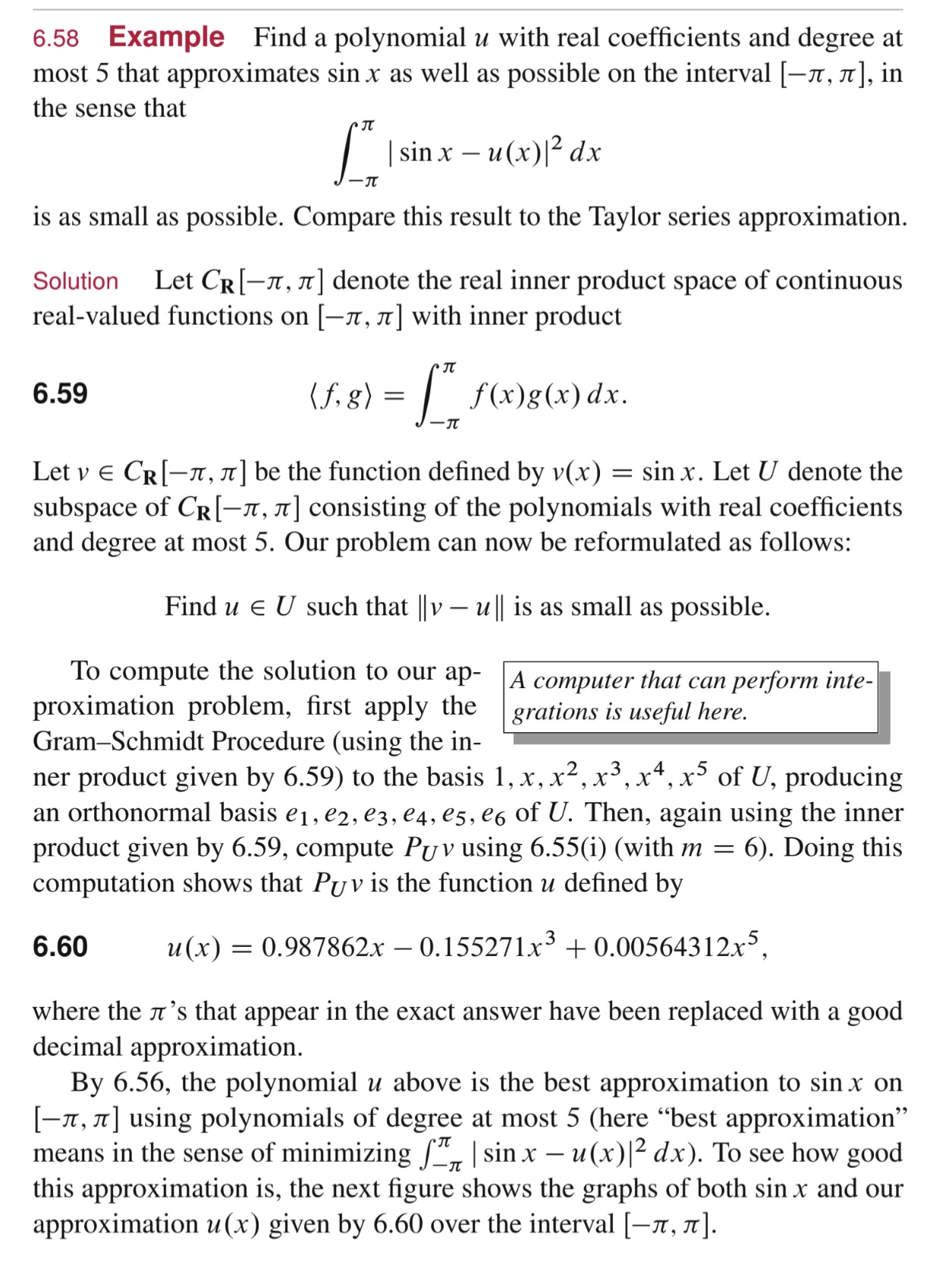
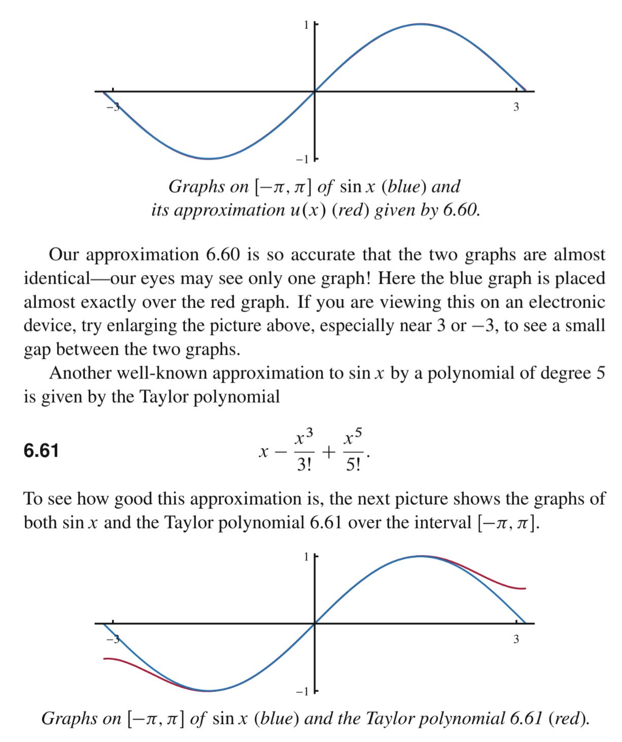
Using Orthonormal Projection to find approximations, even in the space of functions was the coolest. I’ll let Axler speak, it’s mind blowing.

Reisz Representation Theorem was the 2nd coolest: Every finite dimensional linear function φ: V->f has a vector w such that φ(v) = <v,w>. This seems a little obvious if you’re only imagining functionals as “rulers” on a specific basis: given a vector you decide how much each component should could and then sum the entries weighted by your functional. eg. thinking of φ in R^3 as φ([1,2,3]) = f(1) + g(2) + h(3) linear functions f,g,h that map 0 to 0 can only be expressed as a1 + b2 + c*3. That’s clearly a multiplication with another vector in R^3. But when <> represents integration from 0 to 1 with the product of cosine and V is Polynomials up to degree 5, that’s crazy.

You can solve the Fibonacii sequence via expressing it as a linear operator, taking the eigenvalues, then computing the exponent in log multiplications by representing the multiplications in binary.

Every operator can be expressed by polar decomposition, and there’s an extension to linear maps. Explains why a transpose can make sense as an approximation for the inverse, if all eigenvalues about 1.

Can rotate Every operator so that any vector v is mapped to at most 2D subspace, and these 2D subspaces have at most 2 1-D subspaces overlap. Every Normal complex or Self Adjoint (Hermitian, symmetric if real) real matrix is diagonalizable Every Complex matrix is Jordan diagonalizable Ever real matrix has a complexification that is diagonalizable, which means can be expressed in blocks of [[a,-b], [b,a]] with b > 0 Every matrix is diagonalizable if you represent it with different input and output basises

Every matrix in C/with basis of eigenvectors is can be represented as a diagonal matrix, but since eigenvectors aren’t orthogonal, it’s not ‘diagonalizable". np.diag(eigenvalues) = eigenvectors ^-1 @ A @ eigenvectors

Concepts Not Covered

1. Gaussian elimination, instead the ‘row reduction algorithm’. not implied how you can use Gaussian elimination to compute the determinate

2. Regression: The geometric perspective of regression as projecting points was useful to me:

    matrix X is N rows/data-points and P predictors
    matrix Y is N rows, a point
    B is all possible predictors/coefficients
    β is best predictor/coefficients
   
    In Y's space of dimension N, we want to find the vector in the P dimensional hyperplane that is closest to point Y.
   
    It's a P-d hyperplane because X@B has P coefficients in B, and those coefficients can take any values.
   
    The distance from plane X@B to point Y is minimized when the projection of Y onto vector X@β is orthogonal to vector X@β. (That is the error vector vector should go from Y to the tip of X@β)
   
    Orthogonal when X.T@(Y-X@β)=0 implies β = (X.T@X)^-1@X.T@Y
   

Alternatively you want to solve y=Xβ. You can’t do X^-1Y=β since X might not be invertible. Instead multiply by X.T, and for every full rank matrix X, X.T@X is invertible you can now invert that. This is an example of the trick “apply the thing to itself”. X.T@y = X.T@x@β -> (X.T@X)^-1 @ X.Ty = β

3. SVD minimizes all norms that are invariant under unitary transformations by Eckart-Young-Mirsky theorem.
4. More Practical matters such as: 4a. High dimension vectors are almost always nearly orthogonal and can be efficiently embedded in a lower dimension 4b. PCA

Solving the Exercises

The questions are all “easy”, as long as you look over the theorems, but need to check carefully for every subtlety. Having a solutions manual to compare to was great: 1. Just “proving” theorems isn’t enough. If I’ve written a proof I assume it’s correct, so it’s good to catch exactly what I missed. 2. I learned how to write cleaner proof’s and with new techniques. Solution sources: https://linearalgebras.com, https://github.com/jubnoske08/linear_algebra, https://github.com/celiopassos/linear-algebra-done-right-solutions Having good solutions will be a big factor in which textbooks I chose going forward.

If you do every problem sequentially then they’re almost all 1 step proofs. There’s 1 thing to figure out and then you’re done.

My processes was to read all the theorems in the subchapter, think about which theorem to apply and apply it. Then search for a geometric intuition of any new objects. When I used the techniques of the proofs in the chapter, most of the problems are trivial. But it was much harder when I used techniques I’d been more exposed to in the past: sums over elements, geometry of operations, and extending the processes as if I was acting on matrices.

I made it harder by going through and doing every 3rd problem without even looking at the previous two problem statements. If the book is easy because you only have to make 1 logical inference at at a time then skipping problems makes you have to chain together inferences. eg. Normally problems 8,9,10 are all related, and 10 is hard on it’s own. It takes 2 logical inference to solve 10 based on what you know. But if you see the problem statement for 8 and 9 now you have a path to prove 10; problems 8 and 9 provide 1 of the logical inferences you need to solve 10. Once you’ve assumed 8 and 9 are true then you only have 1 more inference to make. I did end up doing every problem. There’s a compounding effect: as you do more you get so by the end I had an intuitive understanding of all the objects I could think of the proof in about as long as it took to write.

There are a few ideas and you just keep applying them.

The Algebraic Tricks:
	apply an operator to itself
	keep applying different operators multiple times
	use the same vector twice
	u=u-a*v + a*v. For what 'a' does this help you?
	try swapping the order:
		for operators ST to TS
		<u1,v1> to <v1,u1>

The Ideas:
	Represent complex numbers as matrix with a+ib=[[a,b], [-b,a]]
	define the new operator/poly as a tweak of the old operator/poly
	summing everything if that's how I can ‘use’ a constraint
	create a subspace <v,T(V),..> where a constraint isn’t true.
	(T-λI) is a null operator if you only look at it acting on the eigenvectors of λ.
	With generalized eigenspaces there's a lot of T^(i-1)T^i counting arguments, understanding how it acts on each direct sum

The Hardest part is when I mis-remembered something I’d learned previously.

1. eg. Min Poly/Char poly can’t categorize matrix, since the jordan blocks for the same eigenvalue could be different. eg dim=4, only λ=1. Could have 2 2d jordan blocks or 1 4d block or 4 1d blocks.
2. Gaussian elimination changes determinant by product. (But it’s an easier way to find determinant: you remember the operations you’ve performed and then multiply the final determinate of either 1 or 0 by all the changes you had to make)
3. SVD sometimes changes which letter “S” represents across authors.
4. “orthogonal” matrices are composed of orthonormal vectors.

But Overall I wish had harder problems to check I’m not only learning shallow correlations. If I only get stuck when something I memorized conflicts with something else then it shows I’m memorizing surface level attributes and not the structure. I also wish I had more practice at finding and extending analogies. eg if Normal matrices are Z, what do non-normal matrices correspond to?